Functorial persistence

The goal of this post is to overcome some hurdles encountered by Bauer and Lesnick. In their approach, some geometric information is lost in passing from persistence modules to matchings. Namely, if an interval ends, we forget if the  $k$-cycle it represents becomes part of another $k$-cycle or goes to 0. Recall:

• $(\R,\leqslant)$ is the category of real numbers and unique morphisms $s\to t$ whenever $s\leqslant t$,
• $\Vect$ ($\BVect$) is the category of (based) finite dimensional vector spaces, and
• $\Set_*$ is the category of pointed sets.

We begin by recalling all the classical notions in the TDA pipeline.

Defintion: A persistence module is a functor $F:(\R,\leqslant)\to \Vect$. The barcode of a persistence module $F$ is a collection of pairs $(I,k)$, where $I\subseteq \R$ is an interval and $k\in \Z_{>0}$ is a positive integer.

Crawley-Boevey describes how to find the decomposition of a persistence module into interval modules. The $k$ for each $I$ is usually 1, but is 2 (and more) if the same interval appears twice (or more) in the decomposition. A barcode contains the same information as a \emph{persistence diagram}, though the former is drawn as horizontal bars and the latter is presented on a pair of axes.

Definition: A matching $\chi$ of barcodes $\{(I_i,k_i)\}_i$ and $\{(J_j,\ell_j)\}_j$ is a bijection $I'\to J'$, for some $I'\subseteq \{(I_i,k_i)\}_i$ and $J'\subseteq \{(J_j,\ell_j)\}_j$.

We write matchings as $\chi\colon \{(I_i,k_i)\}_i \nrightarrow \{(J_j,\ell_j)\}_j$.

Definition: A filtered persistence module is a functor $F:(\R,\leqslant) \to \BVect$ for which $F(s\leqslant t)(e_i) =f_j$ or 0, for every $e_i$ in the basis of $F(s)$ and $f_j$ in the basis of $F(t)$.

The notion of filtered persistence module is used for a stronger geometric connection. Indeed, for every filtered space $X$ the persistence module along this filtration is also filtered (once interval modules have been found), as then inclusions $X_s\hookrightarrow X_t$ will induce isomorphisms in homology onto their image. That is, a pair of homology classes from the source may combine in the target, but if the classes come from interval modules, a class from the source can not be in two non-homologous classes of the target.

Remark: The above dicussion highlights that choosing a basis in the definition of a persistence module already uses the decomposition of persistence modules into interval modules.

It is immediate that a morphism of persistence modules is a natural transformation. Let $\BPVect$ be the full subcategory of $\BVect$ consisting of elements in the image of some filtered persistence module (the objects are the same, we just have a restriction of allowed morphisms).

Definition:  Let $\mathcal B$ be the functor defined by \[ \begin{array}{r c l}
\mathcal B\colon \BPVect & \to & \Set_*, \\
(V,\{e_1,\dots,e_n\}) & \mapsto & \{0,1,\dots,n\}, \\
\left(\varphi:(V,\{e_i\}) \to (W,\{f_j\})\right) & \mapsto & \left(
i \mapsto \begin{cases}
j & \text{ if } \varphi(e_i) = f_j, \\ 0 & \text{ if } \varphi(e_i)=0 \text{ or } i=0.
\end{cases} \right)
\end{array} \]

The basepoint of every set in the image of $\mathcal B$ is 0.

Definition: Let $F,G$ be persistence modules and $\eta$ a morphism $F\to G$.

• The persistence diagram of $F$ is the functor $\mathcal B\circ F$.
• The matching induced by $\eta$ is the natural transformation $\mathcal B(\eta): \mathcal B\circ F\to \mathcal B\circ G$.

Bauer and Lesnick's definition of "matching" allow for more freedom to mix and match barcode intervals, but this also restricts how much information of a persistence module morphism can be tracked.

Example: The following example has a horizontal filtration with the degree 0 homology barcode on the left and the degree 1 homology barcode on the right. Linear maps of based vector spaces have also been shown to indicate how homology classes are born, die (column of zeros), and combine (row with more than one 1).

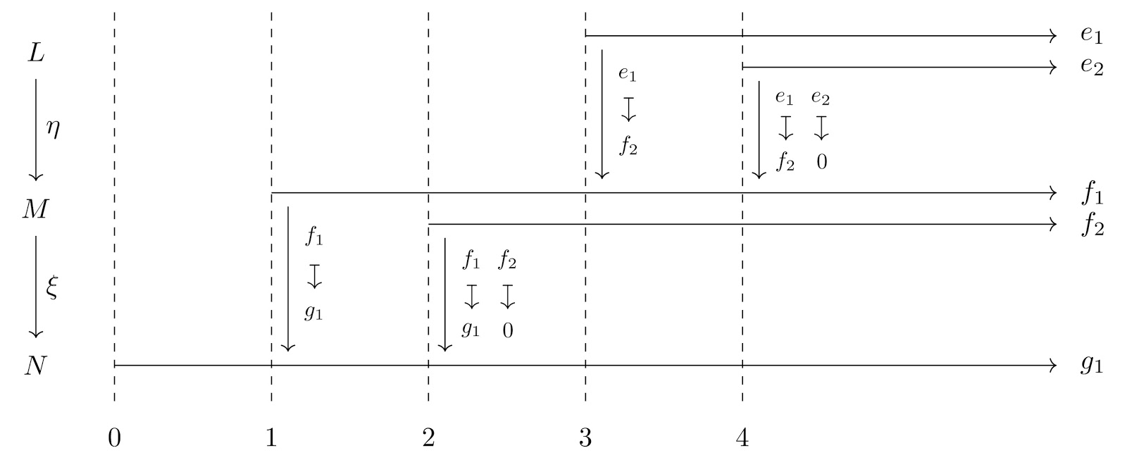
Example: Bauer and Lesnick present Example 5.6 to show that functoriality does not work in their setting. We reproduce their example and show that functoriality does work in our setting. Note that vertical ordering of the bars does not matter once they are named.

Apply the functor $\mathcal B$ to the whole diagram to get the matchings induced by $\eta$ and $\xi$, as below.

Next we hope to understand how interleavings fit into this setup.

References: Bauer and Lesnick (Induced matchings and the algebraic stability of persistence barcodes), Crawley-Boevey (Decomposition of pointwise finite-dimensional persistence modules)

Revisiting persistent homology

Here we revisit and expand on persistent homology, previously in the post "Persistent homology (an example)," 2016-05-19. All homology, except where noted, will be over a field $k$, and $X$ will be a topological space. Often a Morse-type function $f:X\to \R$ is introduced along with $X$, but we will try to take a more abstract view.

Definition: The space $X$ may be described as a filtered space with a filtration of sublevel sets
\[ \emptyset = X_0 \subseteq X_1\subseteq \cdots \subseteq X_m = X, \] whose persistence module is the (not necessarily exact) sequence
\[ 0 = H(X_0) \to H(X_1)\to\cdots \to H(X_m) = H(X) \] of homology groups of the filtration.

Remark: Every persistence module may be uniquely decomposed as a direct sum of sequences $0\to k\to \cdots\to k\to 0$, where every map is $\id$, except the first and last. The indices at which each sequence in the summand has its first and last non-zero map are called the birth and death of the homology class represented by the sequence.

In some cases a homology class may not die, so we consider the extended persistence module to make everything finite. We introduce the superlevel sets $X^i = X\setminus X_i$. If $f$ was our Morse-type function for $X$, with critical points $p_1<\cdots<p_m$, then for $t_0<p_1<t_1<\cdots<p_m<t_m$, we set $X_i = f^{-1}(-\infty,t_i]$ and $X^i = f^{-1}[t_i,\infty)$. The extended persistence module of $X$ is
\[
0 = H_k(X_0) \to H_k(X_1)\to\cdots \to H_k(X_m) \to H_k(X,X^m) \to H_k(X,X^{m-1}) \to \cdots \to H_k(X,X^0)=0.
\]
Definition: The persistence of a homology class in a persistence module conveys the idea of how long it is alive, presented by a persistence pair.

The persistence of all homology classes in a persistence module is often presented in a persistence diagram, the collection of persistence pairs $(i,j)$, or $(p_i,p_j)$ or $(f(p_i),f(p_j))$, as desired; or a linear barcode, the collection of persistence pairs $(i,j)$ as intervals $[i,j]$, ordered vertically. 

Example: Let $X = T^n=(S^1)^n$ be the $n$-torus. One filtration of $X$ is $X_0=\emptyset$ and $X_i = T^i$ for $1\leqslant i\leqslant n$. Note that $H_k(T^n,T^n\setminus X_n)=H_k(T^n)$ and $H_k(T^n,T^n\setminus X_0)=H_k(\emptyset)$. The first $n+1$ modules of the extended persistence module at level $k$ split into $\binom nk$ sequences, as $H_k(T^n) = \Z^{\binom nk}$. Geometric considerations allow $X^i = T^n\setminus T^i$ to be simplified in some cases. For instance, when $n=3$ and $k=0,1$ we have that $\widetilde H_k(T^3,T^3\setminus T^2)\cong \widetilde H_k(T^3,T^2) \cong \widetilde H_k(T^3/T^2)$, and knowing that $X^1=T^3\setminus T^1\simeq (S^1\vee S^1)\times S^1$, the relevant part of the long exact sequence for relative homology is

The two 1-cycles from $S^1\vee S^1\subset X^1$ map via $f$ to the same 1-cycle in $T^3$, hence $\text{im}(g)=\Z^2$. By exactness, $\text{ker}(g)=\Z^2$, and as $g$ is surjective, $A=\Z$.  Hence the extended persistence $k$-modules decompose as 

The persistence pairs are $(1,3)$ with multiplicity 2 and $(2,3)$, $(3,1)$ with multiplicity 1. The persistence diagrams and barcodes of the degree 0 and 1 homology classes are given below.

The diagonal $y=x$ is often given to indicate how short a lifespan a class has. Barcodes are usually not given for extended persistence diagrams, as length of a class (birth to death) is less important than position (above or below the diagonal).

Now we consider some generalizations of the ideas presented above.

Remark: A filtration can also be viewed as a diagram $X_0 \to X_1 \to \cdots \to X_m$, where each arrow is the inclusion map. We could generalize and consider a zigzag diagram, a sequence $X_0 \leftrightarrow X_1 \leftrightarrow \cdots \leftrightarrow X_m$, where $\leftrightarrow$ represents either $\to$ or $\leftarrow$. Homology can be applied and the resulting seuquence can also be uniquely decomposed into summands $k \leftrightarrow \cdots \leftrightarrow k$ where every arrow is the identity, giving zigzag persistent homology.

Remark: A filtration could also be viewed as a functor $F:\{0,\dots,m\}\to \text{Top}$, where $F(i)=X_i$ and $F(i\to j)$, for $j\>i$, is the composition of maps $X_i\to \cdots \to X_j$. Hence the degree-$k$ persistent homology of $X_i$ can be defined as the image of the maps $H_kF(i\to j)$, for all $j\>i$, and the functor $H_kF:\{0,\dots,m\}\to \text{Vec}$ may be viewed as the $k$th persistence module. This is a categorification of persistent homology.

Remark: A space $X$ can be filtered in several different ways. A multifiltration $X_\alpha$, for $\alpha$ a multi-index, is a collection of filtrations such that fixing all but one of the indices in $\alpha$ gives a (one-dimensional) filtration of $X$. The multidimensional persistence of $X_\alpha$ is a $|\alpha|$-dimensional grid of homology groups, with the barcode generalizing to the rank invariant, a map on the grid.

Another generalization, viewing filtrations as quivers, will not be discussed here, but rather presented as a separate post later.

References: Edelsbrunner and Morozov (Persistent homology: theory and practice), Carlsson, de Silva, and Morozov (Zigzag persistent homology and real-valued functions), Bubenik and Scott (Categorification of persistent homology), Carlsson and Zomorodian (The theory of multidimensional persistence)